Useful applications of CNC include making a number of holes around a circle of certain pitch circle diameter (PCD) and machining around the inside or outside of regular polygons. These functions are remarkably similar, each requiring movement in turn to the first vertex, on to the second etc, and on to the last. Given the size (diameter or radius), number of points, start angle and position data, a simple method for working out the coordinates of the vertices is to use the 'polar to Cartesian conversion' within a subroutine loop set to repeat for the number of points. Carefully written, this code will be easily reusable and may be cut-and-pasted into larger programmes.

Fig 407 shows code for one possible implementation of a PCD function. Here the PCD subroutine to call from some encompassing higher-level programme is named 'O 2500'. This is called and executed once per complete PCD operation set. It does little, merely making local copies of the PCD radius (rather than diameter) and the angle for the first hole (or other PCD operation) before calling the next layer down in the subroutine hierarchy, 'O 2501' with the 'L' code to cause its repetition some number of times, once per hole or operation.

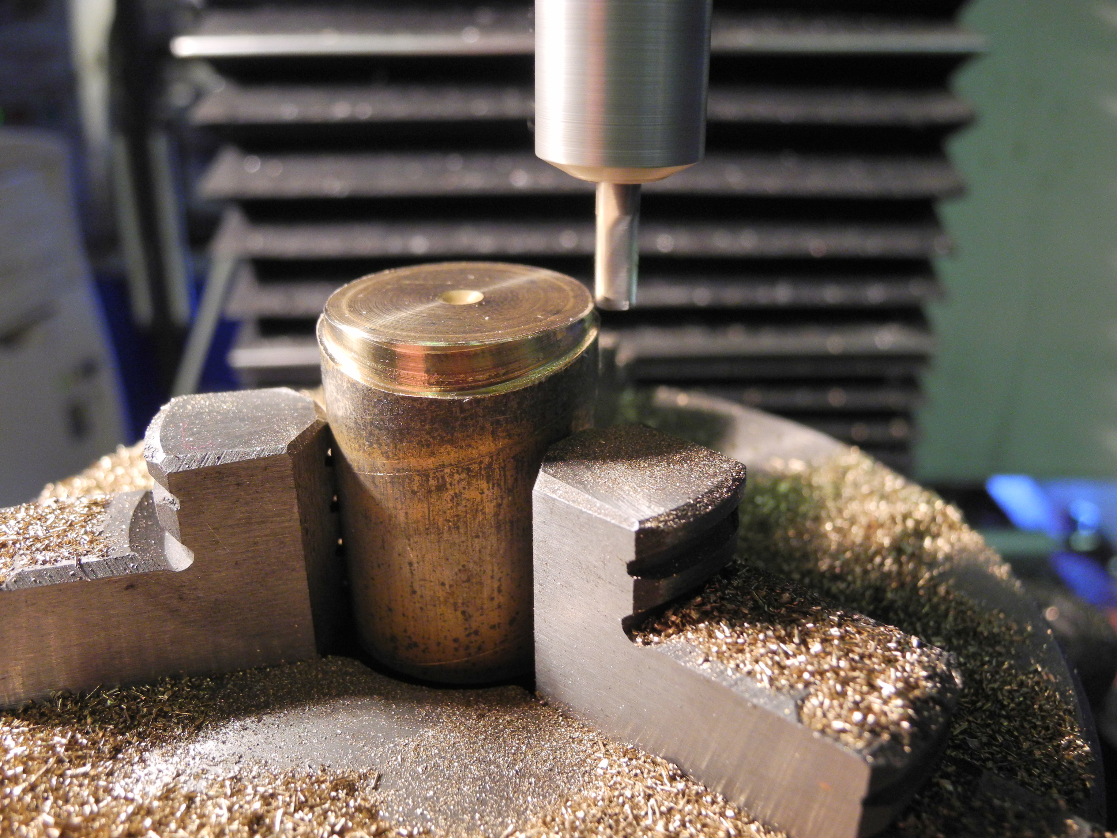
The 'O 2501' subroutine could include all the cutting action, but as written it contains none. Instead, it contains a line to call another subroutine 'O2502' which moves to the new point, lowers and then raises the tool. This nest of subroutines then provides the standard PCD hole-drilling function. But note the extra subroutine 'O2503'. This includes a call to subroutine 'O 2000' from an earlier issue, the 'Hole Mill' function. Other short, simple subs could be written for other purposes, to mill along the sides of a polygon for example, and then hooked into use by the editing of a single line within 'O2501'.

Fig 409 shows a Mach3 plot from a larger programme list written to include 'Hole Mill', the code of Fig 407, and the start-up preamble. Here the PCD code is called twice, once to make four small holes and the second time to make eight larger holes. The 'O 2503' code is included in both cases to cause the PCD code to call the 'Hole Mill' code a total of twelve times. Including a full listing for this would take more than a whole printed page, but it can be found on the accompanying web site www.jons-workshop.com

This demonstrates some of the benefit of designing code to be easily reusable. Building a library of such functional subroutines that can be plugged together in a number of ways is one route to productivity with CNC.

The topic of G code 'modes' will be covered in due course, but to begin with, a cautionary tale. Near the top of subroutine 'O 2501' in Fig 407 note the inclusion of code lines implementing the classic polar to Cartesian coordinate conversion. Regular users of Mach3 G code might imagine we've missed a trick here. Claims have been made that tasks such as PCD drilling can be done “more easily” using the 'G16' code to switch into polar (and out of Cartesian) coordinate system mode. For almost everything we are likely to want to do with a CNC machine we know the X, Y and Z coordinates of where we're going to (and if we don't know, then perhaps we should). This is why we routinely use the Cartesian coordinate system in terms of X, Y and Z to specify our moves. The line:

G1 X2.5 Y-3.0

would seem to mean, quite unambiguously, “move the controlled point in a straight line in the XY plane to the point where X = 2.5 and Y = -3.0 leaving any unspecified axes stationary.”

However, if 'G16' is used to switch Mach3 into 'Polar Mode' beforehand, this same line now means something entirely different. Having entered the 'G16' polar mode (it persists in this mode until cancelled by the G15 code), the 'X' and 'Y' terms get hijacked into meaning 'Radius' and 'Angle'. It can not be over-emphasised that in any programme list, particularly one for controlling machines where safety is a factor, the idea of allowing any one line of code to have more than one entirely different meanings is not only a bad idea, it is one that's hard to beat in terms of badness!

Once this kind of dangerous nonsense is allowed into any listing it becomes more difficult to read, understand and maintain. Certainty about what a simple 'G1' line is for and what it does will be forever in doubt, and will now come with the added requirement of searching back from the beginning of the code to gain certainty as to which mode is active. When running a simulation results in a screen-full of scribble instead of the intended sleek design, how much time will be wasted trying to find that missing 'G15' to get back to 'Cartesian Mode'? G15/G16 is not part of the original EIA 'Standard' 274-D specification for G code, some manufacturers implement it while others do not, and there is no consistency between implementations that do exist – one of the great things about 'Standards', always plenty to choose from!

Long ago when G code emerged as the de facto programming language for numerically controlled machines, programme list storage space was at a premium because programmes were stored as holes punched into a paper tape (Fig 700). Each row across the tape width consisted of a pattern of holes and lack of holes, readable as a binary representation of a character. Various formats existed using different numbers of holes and tape widths, but one popular format used one inch wide paper tape, eight holes across the width for data encoding, and a ninth for engagement with a tractor drive sprocket. Each row across corresponded to one character, or in today's computer terms one 'byte'. With the row spacing fixed at 0.1 inch, nearly three yards of tape was needed to store one kilo byte (1kb = 1024 bytes). For anyone who enjoys gratuitous arithmetic, this makes an interesting comparison to the storage capacity of an '8Gb' (eight giga-byte) memory stick which at today's prices can be bought for about the same price as a pint of beer at the local pub. Storing eight giga-bytes of data on a paper tape would consume almost fourteen thousand miles of tape, enough to stretch more than half way around the equator. This illustrates how important code compactness once was, and how unimportant it is today. Why this matters to us is just because it is often possible to write very compact G code we don't need to, and it is often better to create longer but more readable code – and it is always better to include as much additional comment as you need to make sense of what you're trying to do.

The original code compactness requirement influenced the design of 'modal behaviour' in G code. Consider the two means available in G code for initiating straight line moves, G0 (G Zero) for moving rapidly and G1 (G One) for movement at set feed rate. We have already seen that for G0 and G1, the format of a line is :

G0 X? Y? Z?

where '?' represents numeric values or expressions to be inserted, and where all axis specifiers are optional except at least one must be present. This means that with a simple 3 axis CNC machine such as the Sieg KX1 or KX3 we can programme a straight line move along any one axis, a move along some diagonal across any one plane moving two axes together, or a move from one point in 3D machine space in a straight line to any other by moving all three together.

As part of the 'modal' behaviour, the 'G0 mode' remains active until it is explicitly changed. This was useful when code compactness was an objective. For example to initiate a sequence of three axis moves one after the other we could write:

G0 X10

Y-2.5

Z3

This consumes only eighteen bytes including the essential but unseen 'LF' (line feed) and 'CR' (carriage return) control characters at the end of each line, and would occupy 1.8 inches of paper tape. Because G code is executed one line at a time, this would cause a sequence of up to three rapid movements – firstly moving the X axis to coordinate +10.0, next the Y axis to coordinate -2.5 and finally Z to +3.0. However, if this is really what we intend, it makes for much easier reading to write:

G0 X10 ; Comment

G0 Y-2.5 ; Comment

G0 Z3 ; Comment

Both representations result in exactly the same movement sequence with the 'G0 rapid move' mode remaining active. Particularly when using the Mach3 'MDI' (Manual Data Input) feature, it might be safer to follow a G0 move with a G1 move at the slower feed speed to leave the 'G1' mode active instead. The above 'G0' sequence could be followed by:

G1 X10 ; Into slower move mode

This causes no further movement as the axis is already at the position, however it leaves the mode in the slightly safer 'G1' condition.

Mach3 may be in several modes at the same time, but only one mode from each 'modal group' may be active. G0 and G1 are both members of 'Modal Group One – Motion' which also contains arc movement commands G2 and G3 amongst others. Other modal groups include 'Group Two - Plane Selection' which includes codes G17, G18 and G19. These select the current working plane as the XY plane (used for most of what we do), the XZ or the YZ planes respectively, clearly we can only be working in one of these at a time. Group six contains only G20 and G21 which determine working units as inches or metric (mm).

The Mach3 documentation fully explains these and all other modes and modal groups, however there is one more to mention here as it is one that some machinists choose to use almost all of the time while others use it never, the 'Group Seven - Cutter Radius Compensation'. This mode group uses codes G40 to turn cutter radius compensation off, G41 turns compensation on such that the cutter travels a path one tool radius to the left of the programmed path, likewise G42 for the tool to the right. This makes it a simple matter to cut around the outside or the inside of a shape saving the trouble of generating code for a tool path one tool radius removed from the finished part boundary. It sounds simple, but thought will be needed to plan in some extra moves upon entering an offset compensation mode – not unlike a pilot lining up his flight path with the runway before attempting a landing. Once the cut has completed, it is all too easy to forget to switch back out of compensation mode and again, some extra lining-up moves will be needed to restore order after a 'G40'.

Mach3 will almost always produce the correct tool path in these offset modes, but on rare occasions and for no obvious reason, you might find the odd extra half-moon of material has been gouged out. This is because implementing cutter radius compensation is far more difficult than you might at first imagine. Suppose, for example, the tool is proceeding along to the left on a straight but approaching a corner. How far to proceed in the current direction depends upon whether the turn at the corner is to the right or the left, and at what angle. Then there are a choice of strategies. Should the tool path move around sharp corners by moving in straight lines or should it move in an arc of tool radius around the corner. But what if the next move is an arc of radius less than the tool radius? And what if further along in the cutting sequence the tool passes near this point again? Some 'Look Ahead' strategy is also needed – so perhaps we can forgive Mach3 these occasional failings, it is after all a hugely complex piece of software that does almost everything else safely and 'as advertised'. For many simple jobs it is easy enough to avoid the offset modes 'just in case' by including a tool radius parameter in our programme listing and then for us to take responsibility for driving the tool path where we want it. In some cases – where we might want to machine around the inside or the outside of some shape for example – we could use a positive radius to machine around the outside and a negative value for radius to machine around the inside. With most machining problems alternative methods exist.

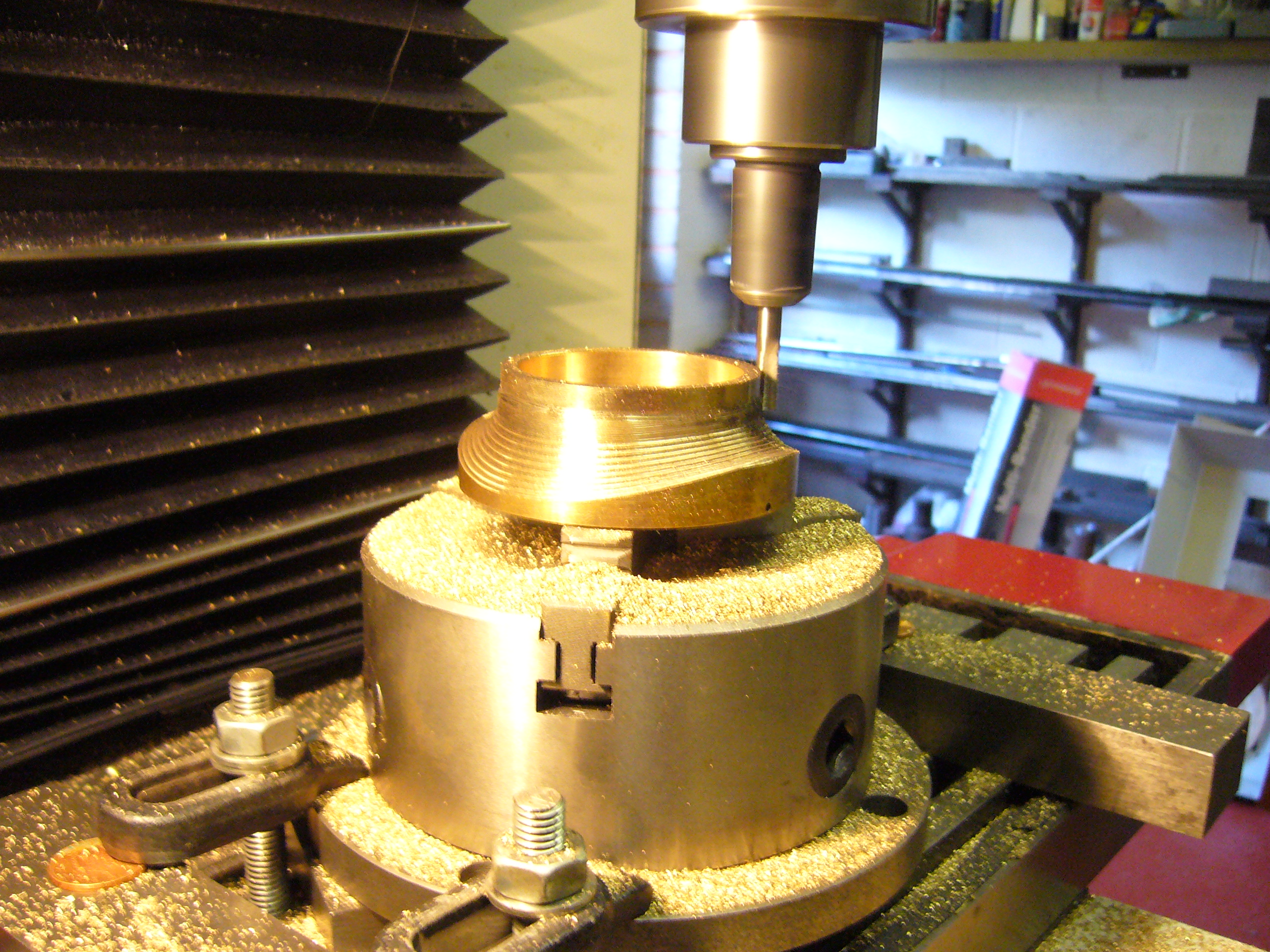
Knowing that G2 and G3 can be used to cut arcs and that a new 'Z' coordinate may be specified causing the end of the arc (in the XY plane) to be at a new height 'Z', this suggests making up an undulating circle from some number of connecting arcs, each finishing at a height appropriate to its position – see Fig 410 machining a chimney base upper surface.

In choosing some number of arcs, 'Arcs_per_Circ', this wants to be large enough that joins between arcs are not obvious, some number around one hundred may be a good starting point but we will make a point of writing the code to be easily modifiable, placing our chosen 'Arcs_per_Circ' figure in a single parameter somewhere obvious near the start of the code.

Determining the X and Y coordinates of the vertex at the end of each of these small arcs is a problem we have solved previously, this is the familiar PCD (pitch circle diameter) problem, the core of which shakes down to the standard polar to Cartesian conversion:

For circular or other symmetrical shapes, it is often helpful to define the XY origin (where X = 0.0 and Y = 0.0) at the centre of the work-piece. This allows some simplification of the arithmetic, the 'Centre X' and 'Centre Y' offset values used in the polar to Cartesian conversion, for example, become zero and so drop out of the arithmetic.

For cutting arcs using 'G2' or 'G3' we have the choice of using 'Centre' or 'Radius' formats. Full descriptions of these may be found in the Mach3 documentation and elsewhere, and it is generally accepted that centre format is preferred, as unlike radius format, it produces accurate results for all angles up to and including the full circle. However, for small angles the radius format remains good, and being slightly easier to use, will be used here. Radius format use for 'G2' or 'G3' is:

G2 X? Y? Z? R? ;

where '?' represents numeric values or expressions to be inserted.

This code will be designed to cut around one complete circle, using the number 'Arcs_per_Circ' of G2 (or G3) arc movements. With no reason to choose otherwise, the angle of the start point will be chosen as zero degrees (3 o'clock, or east). The repetition involved suggests a 'loop' code structure, this implies the code will consist of (at least) two subroutine levels – the first level routine called from a higher level, and a second level subroutine (or sub-subroutine if it helps to look at it that way) will be used to perform the repetitive inner 'loop' function. Fig 411 is a geometric sketch to help clarify our thinking. The 'Plan view' shows the axis of the large tube of radius 'S' being horizontal or aligned with the CNC milling machine X axis.

A start may now be made on writing a pseudo-code. The first level subroutine needs four figures to work with, these are the bush radius 'R', boiler radius 'S', tool radius 'T', and 'Arcs_per_Circ'. In addition to these four, and thinking ahead, it would be useful to create code which would work either way up – to machine something such as a chimney base from above, as well as machining a boiler bush flange from below. Including some 'Gain' value which may be given values of plus one for cutting from above, or minus one for cutting from below, would allow for this. Of course in including this, we are free to use any other value for gain.

A usable pseudo-code might be:

;**Undulating Circle Pseudo-Code**
;**For cutting boiler bush flanges,
;**chimney and dome bases and similar
; Requires 5 Parameters set beforehand:
;   'R'  Radius of bush to fit through hole
;   'S'  Radius of boiler or smokebox
;   'T'  Tool radius
;   'Arcs_per_Circ'
;   'G' Gain, usually plus or minus one so
;      that cut works from above or below!
;**
;  Local parameters set-up here
;   'Angle_Step' = 360 / 'Arcs_per_Circ'
;   Angle 'Theta' = 0.0 degrees
;  Tool path radius 'U' = 'R' + 'T'
;**
;  Move to start position X, Y, Z
;  Call 'Arc' Loop,'Arcs_per_Circ' times
;  Lift tool clear of job
;Return	; Have cut undulating circle
;
;** 'Arc' Loop subroutine
;  Theta = [Theta - Angle_Step]
;  Calculate new X, Y and Z
;  Cut arc to new X, Y, Z
;Return	; Have cut one arc
;** Pseudo code End **

Once satisfied the pseudo-code 'works' and makes sense the next task is to come up with the set of arithmetic equations and 'plug them in'. For each iteration around the loop, the new values of X, Y and Z for use in the G2 or G3 arc move are re-calculated using the updated angle around the circle 'Ө, Theta'. Note if the intention is to proceed around the circle in a clockwise direction, the value of 'Theta' will need to become more negative, or less positive, on each iteration of the loop, this explains the “Theta = [Theta - Angle_Step]” in the pseudo-code.

The tool path radius (Q = R + T) is used in the polar to Cartesian conversion equations to find the X and Y coordinates for the G2 or G3. Assuming the centre is point X=0.0, Y=0.0, these reduce to:

X = Q * cos Ө Y = Q * sin Ө

That only leaves the 'Z' value to find. With the tool at any angle 'Ө' around the bush, the distance of the point of cutter contact away from the highest point is shown in Fig 411 as 'y', where, from our knowledge of polar to Cartesian conversion:

y = R * sin Ө

The required depth 'Z' value at this point may then be found using Pythagoras theorem as two sides of the shown right angled triangle are known:

a = √ (S² - y²) d = S - a

Multiplying 'd' by the 'Gain' value selects the desired upward or downward deflection of the Z coordinate.

The value of 'y' takes on positive and negative values, this of course does not upset the Pythagoras calculation as 'y' squared is always positive.

Having calculated the new X, Y and Z coordinates required at the end of the arc, the arc is cut and the 'Arc' loop subroutine is repeated 'Arcs_per_Circ' times. Readers wanting more detail on the maths involved may find it on the companion web site www.jons-workshop.com

Fig 412 illustrates the benefit of checking your work. Insufficient thought during coding led to the decision to add 'Angle_Step' to 'Theta' on each pass through the 'Arc' loop subroutine:

; 'Theta' = ['Theta' + 'Angle_Step];

This of course leads to angle 'Theta' taking on an increasing positive value as it proceeds around the circle which by convention is anti clockwise. This would have been correct if using 'G3' to cut the arcs in an anti clockwise direction. However, it was intended to cut clockwise to take advantage of the better finish that often results from 'climb' milling rather than 'conventional' milling. This error might have gone undiscovered had it not been tried in simulation using an unrealistically small value for 'Arcs_per_Circ'. The problem was easily fixed, replacing '+' with '-' to get 'Theta' going the other way.

The idea of the 'Gain' control allowed setting gain values of +1.0 or -1.0 to cover the uses of cutting a chimney base from above or a bush flange from below, but more useful still, this 'Gain' control may take any value, and it was this useful feature that made it relatively simple to blend the skirt of the chimney base up into a circular section where it meets the main chimney tube.

Fig 413 shows a simulated tool path generated by calling the undulating circle code three times, using 'Gain' values of +1.0, 0.0 and -1.0. The gain of 0.0 produces a flat circle. The final subroutine set is shown in Fig 760. Note it is left to the calling code to position the tool at the start, optionally this could be included in the subroutine. The nominal 'Z' value is assumed to be zero, for practical uses it might be sensible to include code to handle some Z offset value. The finished code used to generate Fig 413 is up on the web site www.jons-workshop.com

It is a simple matter to treat the undulating circle subroutine as a loop to be called from some higher level code any number of times. This might be useful when using a small tool where you might not want to risk ripping off all the material in one pass around. A method would be to reduce the tool height on each pass until the desired depth has been reached.

The chimney base code calls this undulating circle code a number of times with the radius and the gain values altered automatically between circles producing the smooth blend. Code for this is also on the web site.

Looking at Figs 411 and 414 together, is is apparent we can not accurately cut a sloping surface using a vertical, flat ended tool. However, any error is very small at the radius 'R', the deviation caused by not tilting the tool becoming more noticeable towards the outside diameter. For a boiler bush or similar this probably does not matter, this still makes a far better job than a flat flanged bush produced on the lathe, but the deviation may be minimised by using a smaller tool. To cut the flange might then require a number of cuts taking smaller bites. Another idea is to minimise the flange width. As seen previously, the flange serves little purpose other than to seat the bush correctly prior to brazing or silver soldering, contributing little if anything to joint strength.